Google Sheets UNIQUE Function

Syntax of the UNIQUE Function

=UNIQUE(range, [by_column], [exactly_once])

• range: Range is the range of cells which you wish to filter for unique values. This is the only required argument. It can be a one-dimensional range (occupying only one row or column) or a two-dimensional range of cells (occupying multiple rows and columns).
• by_column: By_column is an optional argument that specifies whether you want to filter unique values by column. It defaults to false, which makes sense when filtering a vertical range of cells (i.e. asking the UNIQUE function to return unique rows). If you're ever filtering a horizontal range of cells, you'll want to specify true for this argument so that it returns unique values by column.
• exactly_once: Exactly_once is another optional argument that specifies whether we only want to include values that have no duplicates. It defaults to false, so it will list a duplicate value once. However, if this argument is set to true, it will ignore any duplicate values in the range and only return values that are not duplicated in the range.

Examples of How to Use the UNIQUE Function in Google Sheets

Below are some examples of how to use the UNIQUE function in Google Sheets, starting with the most basic.

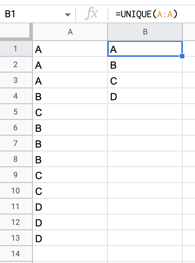
This is the most basic example of using the UNIQUE function in Google Sheets. We have a list of letters in column A and we use the UNIQUE function =UNIQUE(A:A) in cell B1 which returns a list of all unique values in the range (column A) in the order in which they first appear. Note that the result is not contained to one cell like we often see with functions; instead Google Sheets starts the result where we typed the formula and then populates the results downwards toward the bottom of the spreadsheet, occupying as many rows as there are unique rows in the result.

Using UNIQUE on a Horizontal Range of Cells

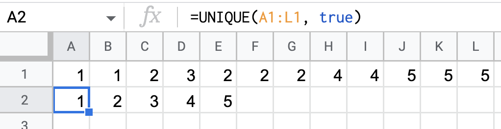
This example shows how to use the UNIQUE function =UNIQUE(A1:L1, true) to filter a horizontal range of cells in Google Sheets. We have to set the by_column argument to true so that it looks for unique values by column and not by row. If we omitted this argument it would default to false, and would simply consider the horizontal range A1:L1 to be one long unique row, and would simply return the same range.

Using UNIQUE to Return Unique Rows Across Multiple Columns

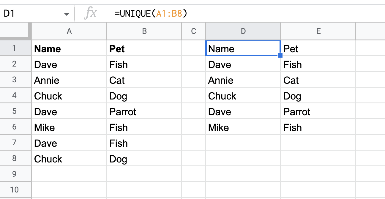
In this example, we are using Google Sheets to organize a list of our friends' pets, and want to make sure we only have unique values in the list. This is a two-dimensional range, because we want unique combinations of name and pet. By typing the formula =UNIQUE(A1:B8) into cell D1, we get all unique combinations of columns A and B. Because our source range spans two columns, our result range will also span two columns.

Note that one combination of "Chuck" and "Dog" has been removed, because there is a duplicate row in the original range. Also note that one row of "Dave" and "Fish" has also been removed, but not the row with "Dave" and "Parrot." This is because while Dave may be a duplicate in the Name column, our formula is looking for unique rows across both Name and Pet. In other words, the UNIQUE function is looking for unique combinations of all columns included in the range.

Using the UNIQUE Function to Return Only Unique Values and Ignore Duplicates

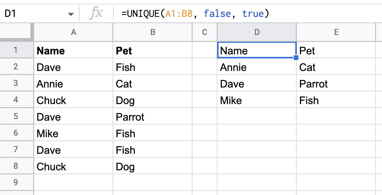
Finally, in this example, we see what happens when we set the exactly_once argument to true. We use the UNIQUE function with the same range of cells but set the by_column argument to false and the exactly_once argument to true: =UNIQUE(A1:B8, false, true). Now rather than including one row of "Dave" + "Fish" and one row of "Chuck" + "Dog," the formula simply omits all of these rows because the exactly_once argument tells Google Sheets that you don't want any duplicate row from the range in your results, not even once.

The UNIQUE Function Takes Up Multiple Cells

Because the UNIQUE Function in Google Sheets returns a range of cells which contain the unique values, it needs enough blank cells (one per unique value) below where you write the formula in order to work. Because it returns a range of cells, this is called an "array result" as opposed to simply returning a value contained in one cell of your spreadsheet. Whenever you write a formula which will return an array result, you need to ensure that it has enough room to display the entire result, otherwise Google Sheets will return a #REF! error.

This means that if you write a formula using the UNIQUE function in cell A1 and there are 5 unique values, then cells A2 through A6 need to be empty so that the function can display the entire array result without overwriting any other data.

#REF! Error From the UNIQUE Function in Google Sheets

The UNIQUE function will return a #REF! error if there is not enough room to display all of the unique results. Ensure that there are enough empty cells below the cell where you wrote the formula to display all of the unique values. See the section above for more details.

Deleting Values Returned by the UNIQUE Function

As mentioned above, the UNIQUE Function returns a range of cells called the "array result." Because all of the cells in the array result are part of one single result, Google Sheets will not let you delete any one cell from the result. If you select a cell in the results and hit the delete key, nothing will happen. In order to remove rows from the results, you will need to delete or modify the formula.

Using the UNIQUE Function With Formatted Data in Google Sheets

Google Sheets lets you format data in a number of ways, but this may lead to confusion when using the UNIQUE function. You may see 1, 100.00%, and $1.00 and believe that they are all unique values, but we need to remember that the underlying value is 1 and that only the format is different. For this reason, Google Sheets treats these as duplicate values and will only return one of them in the results of the UNIQUE function. Also ensure that there are no spaces hiding at the end of text because this will also make Google Sheets think that these are unique values when you want them to be treated as duplicates.

Try Practice Problems With UNIQUE

To fully commit this function to memory you need to get some hands on experience. Try some practice problems with the UNIQUE function in our interactive Google Sheets Tutorial now!